Post Hoc Nearest Neighbors Prediction Adjustments

---

Quinlan (1993) describes a post-processing technique used for numeric predictions that adjusts them using information from the training set.

Let’s say you have some model with a numeric outcome \(y\) and a vector of predictors \(\boldsymbol{x}\). We’ve fit some model to the training set and we have a new observation with predictors \(\boldsymbol{x}_0\); the model’s prediction is \(\widehat{y}_0\).

This method finds the \(K\)-nearest neighbors to \(\boldsymbol{x}_0\) from the training set (denotes as \(\boldsymbol{x}_1\ldots \boldsymbol{x}_K\)) and their corresponding predictions \(\widehat{y}_i\). The distances from the new sample to the training set points are \(d_i\).

For the new data point, the \(K\) adjusted predictions are:

\[ \widehat{a}_i = y_i + (\widehat{y}_0 - \widehat{y}_i) \]

for \(i=1\ldots K\). The final prediction is the weighted average the \(\widehat{a}_i\) where the weights are \(w_i = 1 / (d_i + \epsilon)\). \(\epsilon\) is there to prevent division by zero and Quinlan defaults this to 0.5.

Suppose the true value of the closest neighbor is 10 and its prediction is 11. If our new value \(\boldsymbol{x}_0\) is over-predicted with a value of 15, we end up adjusting the prediction down to 14 (i.e., 10 + (15 - 11)).

This adjustment is an integral part of the Cubist rule-based model ensemble that we discuss in APM (and will later in this book). We’d like to apply it to any regression model.

To do this in general, I’ve started a small R package called adjusted. It requires a fitted tidymodels workflow object and uses Gower distance for calculations.

Here’s an example using MARS on the food delivery data:

library(tidymodels)

── Attaching packages ────────────────────────────────────── tidymodels 1.2.0 ──

✔ broom        1.0.5      ✔ recipes      1.0.10
✔ dials        1.2.1      ✔ rsample      1.2.1 
✔ dplyr        1.1.4      ✔ tibble       3.2.1 
✔ ggplot2      3.5.0      ✔ tidyr        1.3.1 
✔ infer        1.0.6      ✔ tune         1.2.0 
✔ modeldata    1.3.0      ✔ workflows    1.1.4 
✔ parsnip      1.2.1      ✔ workflowsets 1.1.0 
✔ purrr        1.0.2      ✔ yardstick    1.3.1 

── Conflicts ───────────────────────────────────────── tidymodels_conflicts() ──
✖ purrr::discard() masks scales::discard()
✖ dplyr::filter()  masks stats::filter()
✖ dplyr::lag()     masks stats::lag()
✖ recipes::step()  masks stats::step()
• Learn how to get started at https://www.tidymodels.org/start/

# Found at https://github.com/topepo/adjusted
library(adjusted)
# Also requires the earth package

tidymodels_prefer()
theme_set(theme_bw())

The data are in the modeldata package. We’ll do the same split as the book (training/validation/testing):

data(deliveries, package = "modeldata")

set.seed(991)
delivery_split <- initial_validation_split(deliveries, prop = c(0.6, 0.2),
                                           strata = time_to_delivery)
delivery_train <- training(delivery_split)
delivery_test  <- testing(delivery_split)
delivery_val   <- validation(delivery_split)

Let’s specify a multivariate adaptive regression spline model that can utilize two-factor interaction terms. The initial code is pretty simple:

mars_spec <-  
  mars(prod_degree = 2) %>% 
  set_mode("regression")

mars_fit <- 
  workflow() %>% 
  add_formula(time_to_delivery ~ .) %>% 
  add_model( mars_spec) %>% 
  fit(data = delivery_train)

We can use the earth package’s format() function to see the model terms/splits. It’s fairly long though:

mars_fit %>%
  extract_fit_engine() %>% 
  format(digits = 3) %>% 
  cat()

  53
  -  0.456 * dayTue
  +   3.48 * dayWed
  +   5.97 * dayThu
  +   10.6 * dayFri
  +   15.1 * daySat
  +   3.68 * daySun
  -   1.13 * h(hour-16.233)
  -   2.35 * h(17.319-hour)
  +  0.466 * h(hour-17.319)
  -   2.57 * h(3.84-distance)
  +   3.99 * h(distance-3.84)
  -  0.563 * h(2-item_02)
  +   4.22 * h(item_02-2)
  -  0.554 * h(1-item_03)
  +  0.851 * h(item_03-1)
  -   11.6 * h(2-item_10)
  +   10.4 * h(item_10-2)
  -  0.807 * h(1-item_24)
  +  0.581 * h(item_24-1)
  +  0.869 * h(17.319-hour)*dayTue
  -  0.656 * h(17.319-hour)*dayThu
  -   1.57 * h(18.023-hour)*dayFri
  -   1.39 * h(hour-18.023)*dayFri
  -    1.7 * h(18.629-hour)*daySat
  -   2.86 * h(hour-18.629)*daySat
  +   1.16 * h(distance-3.84)*dayFri
  -  0.561 * h(5.02-distance)*daySat
  +    2.1 * h(distance-5.02)*daySat
  -   11.3 * h(1-item_01)*item_10
  +   9.95 * h(item_01-1)*item_10
  -   1.43 * h(1-item_10)*daySat
  -   2.55 * h(item_10-1)*daySat
  -  0.578 * h(17.319-hour)*h(distance-3.54)
  +  0.324 * h(17.319-hour)*h(3.54-distance)
  +   1.05 * h(1-item_01)*h(item_09-1)
  -  0.546 * h(1-item_01)*h(1-item_09)

Warning

I just made the package; it would probably be called “experimental.” The syntax below may change in the future.

The adjusted package requires the use of the fitted model as well as the initial training set. The main function nn_adjust() has those two arguments:

adj_obj <- nn_adjust(mars_fit, training = delivery_train)

and pretty much does nothing at this point. We don’t even need to specifiy the number of neighbors until prediction/adjustment time:

# Predict the first validation row: 
x_0 <- delivery_val %>% slice(1)

# Original prediction:
predict(mars_fit, x_0)

# A tibble: 1 × 1
  .pred
  <dbl>
1  29.1

# Same:
predict(adj_obj, x_0, neighbors = 0)

# A tibble: 1 × 1
  .pred
  <dbl>
1  29.1

# Adjust using 3 most similar samples
predict(adj_obj, x_0, neighbors = 3)

# A tibble: 1 × 1
  .pred
  <dbl>
1  29.5

So how many neighbors should we use? Let’s try different values and compute the RMSE for the validation set:

val_pred <- 
  tibble(neighbors = 0:20) %>% 
  mutate(
    .pred = map(neighbors, 
                ~ augment(adj_obj, new_data = delivery_val, neighbors = .x)),
    rmse = map_dbl(.pred, ~ rmse_vec(.x$time_to_delivery, .x$.pred))
  )

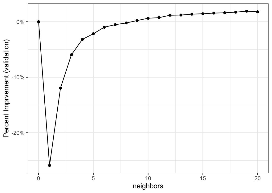
The RMSE profile looks fairly common (based on our experiences with Cubist). The 1-NN model is awful since it is over-fitting to a single data point. As we increase the number of neighbors the RMSE drops and eventually surpasses the results without any adjustment:

val_pred %>% 
  ggplot(aes(neighbors, rmse)) +
  geom_point() + 
  geom_line() +
  labs(y = "RMSE (validation)")

Let’s compute the percent improvement relative to the no-adjustment case:

val_pred_0 <- val_pred %>% filter(neighbors == 0) %>% pluck("rmse")

val_pred %>% 
  mutate(pct_imp = (val_pred_0 - rmse) / val_pred_0) %>% 
  ggplot(aes(neighbors, pct_imp)) +
  geom_point() + 
  geom_line() + 
  scale_y_continuous(labels = scales::percent) +
  labs(y = "Percent Imprvement (validation)")

For these data, the best case is a 1.9% improvement in the RMSE. That’s not a game changer, but it is certainly helpful if every little bit of performance is important.

I made this package because the tidymodels group is finally focusing on post-processing: things that we can do to the model predictions to make them better. Another example is model calibration methods.

Our goal is to let you add post-processing steps to the workflow and tune/optimize these in the same way as pre-processing parameters or model hyperparameters.